Episodic semi-gradient SARSA for on-policy control
Zhihan Yang, September 2 2020
Table of content
- Imports
- Algorithm
- Implement important classes
- MountainCar-v0 example
- Description of the task
- Train agent
- Plot episode lengths over time
- Watch the car climbs the hill (videos))
- Initial position: left of the lowest point
- Initial position: right of the lowest point
- Interpret the learned value function
- Interpret the learned policy
%load_ext autoreload
%autoreload 2
Imports
import json

import numpy as np
import matplotlib.pyplot as plt
import gym

from tqdm.notebook import tqdm

import sys
sys.path.append('../../modules')

import matplotlib.pyplot as plt
from mpl_toolkits.mplot3d import Axes3D
import mpl_toolkits.mplot3d.art3d as art3d

from scipy.signal import savgol_filter

# for video display
import io
import base64
from IPython.display import HTML
from gym import wrappers
Algorithm
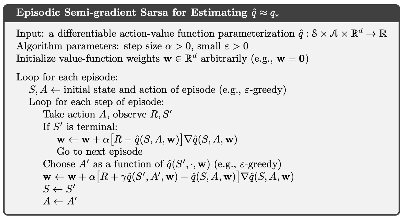
The algorithm below will be implemented in this article. It is basically SARSA adapated to function approximation of the action value function. For the motivation of SARSA and Q-learning, please check out a previous post of mine. For the derivation of the update rule, please check out the section 9.3 Stochastic Gradient and Semi-gradient Methods of Sutton & Barto RL Book.

Implement important classes
Tile coding
Tile coding is a method for constructing discrete features from continuous state spaces. Compared to the naive grid-based approach (converting a continuous state space into a discrete space of non-overlapping grid cells), tile coding allows for generalization and therefore faster learning.
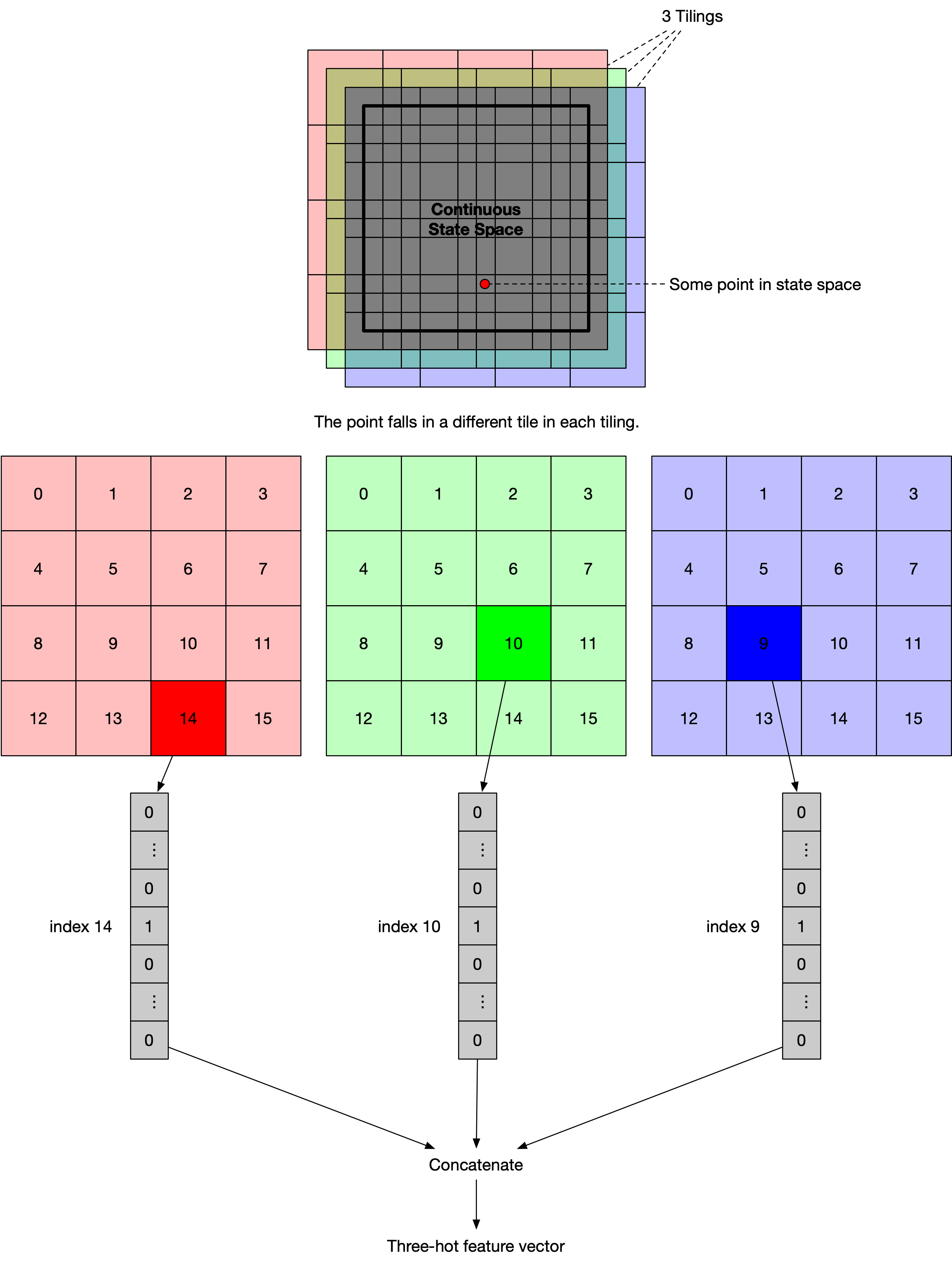
For instance, suppose we have the following 2D continuous state space (the square with bold borders). Then tile coding works as follows:

where each tiling is a mesh of tiles.
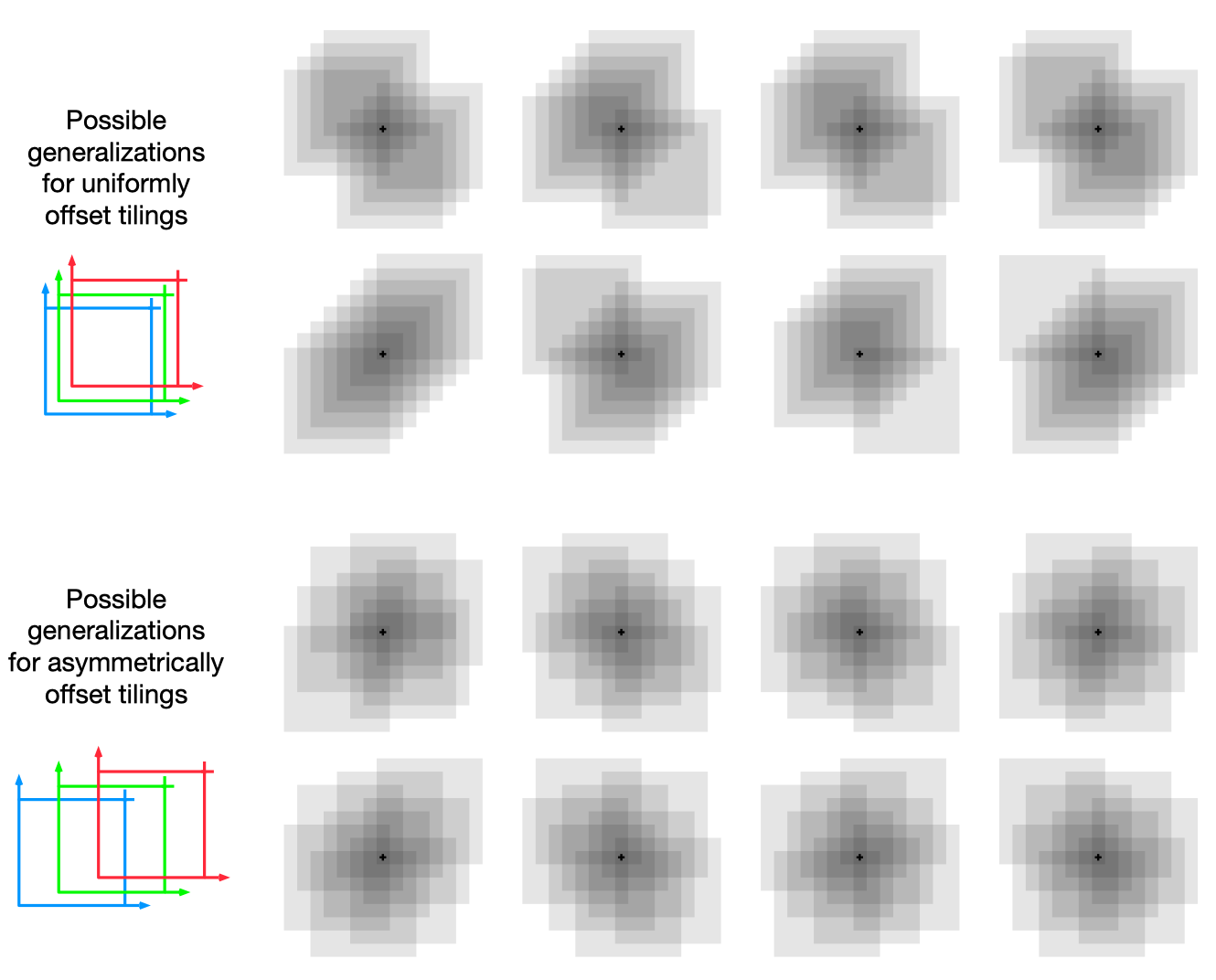
If we are using a linear model with no interaction, then the weights corresponding to exactly these 3 tiles will be updated. This enables local generation because each tile contains a subset of points (not just one) in the state space. In practice, tilings are offsetted asymmetrically because doing so results in spherical generalization, while symmetric tiling results in diagonal generalizations (see the figure below copied from the book). In this implementation, I used random offsets to make things easier.
 Reference: Sutton & Barto RL Book (Page 219)
I've annotated the following code cells to make them as readable as possible. The class Tiling2D is used to create instances of individual tilings which are used in the class Tile2DFeatureConstructor to create the $k$-hot feature vectors ($k$ is the number of tilings).
class Tiling2D:

    """One tiling. """

    def __init__(
        self,
        x_min, x_max, y_min, y_max,
        num_tiles_per_dim,
        x_offset_p, y_offset_p,
    ):
        """
        :param x_min: minimum value of the x dimension
        :param x_max: maximum value of the x dimension
        :param y_min: minimum value of the y dimension
        :param y_max: maximum value of the y dimension

        :param num_tiles_per_dim: (suppose no offsets) the number of partitions for each dimension

        :param x_offset_p: proportion (of the width of a partition) to shift (towards a smaller value along the x dimension)
        :param y_offset_p: proportion (of the width of a partition) to shift (towards a smaller value along the y dimension)
        """

        assert x_offset_p >= 0 and x_offset_p < 1
        assert y_offset_p >= 0 and y_offset_p < 1

        x_tile_width = (x_max - x_min) / num_tiles_per_dim
        y_tile_width = (y_max - y_min) / num_tiles_per_dim

        x_offset = x_tile_width * x_offset_p
        y_offset = y_tile_width * y_offset_p

        # explanation for +1+1:
        # - 1st +1: extra tile to cover the entire state space (after we've shifted the tiling)
        # - 2nd +1: number of bin edges is number of bins + 1
        self.xs = np.linspace(x_min-x_offset, x_max-x_offset+x_tile_width, num_tiles_per_dim+1+1)
        self.ys = np.linspace(y_min-y_offset, y_max-y_offset+y_tile_width, num_tiles_per_dim+1+1)

        self.num_tiles = int((num_tiles_per_dim + 1) ** 2)
        self.num_tiles_per_dim = num_tiles_per_dim

        self.x_max = x_max
        self.x_min = x_min
        self.y_max = y_max
        self.y_min = y_min

    def get_x_bin_index(self, x):
        for i in range(len(self.xs) - 1):
            if (x >= self.xs[i] and x < self.xs[i+1]):
                return i

    def get_y_bin_index(self, y):
        for i in range(len(self.ys) - 1):
            if (y >= self.ys[i] and y < self.ys[i+1]):
                return i

    def preprocess(self, state) -> np.array:
        x, v = state
        # convert from 2d indexing to 1d indexing:
        # bin index = row index (0-based) * number of tiles per row + column index (0-based)
        bin_index = self.get_x_bin_index(x) * (self.num_tiles_per_dim + 1) + self.get_y_bin_index(v)
        return bin_index
class Tile2DFeatureConstructor:

    def __init__(
        self,
        x_min:float, x_max:float, y_min:float, y_max:float,
        num_tiles_per_dim:int,
        num_tilings:int,
        seed:int,
    ):
        np.random.seed(seed)
        self.tilings = [
            Tiling2D(
                x_min, x_max, y_min, y_max,
                num_tiles_per_dim,
                np.random.uniform(), np.random.uniform(),  # np.random.uniform() has interval [0, 1)
            ) for i in range(num_tilings)
        ]
        self.num_features = num_tilings * (num_tiles_per_dim + 1) ** 2

    def preprocess(self, state:tuple) -> np.array:
        feature_vectors = []

        for tiling in self.tilings:
            feature_vector = np.zeros((tiling.num_tiles, 1))
            onehot_index = tiling.preprocess(state)
            feature_vector[onehot_index] = 1
            feature_vectors.append(feature_vector)

        return np.vstack(feature_vectors)  # concatenation
Linear approximator
class LinearApproximator:

    def __init__(self, num_actions:int, lr:float, fc):
        self.lr = lr  # learning rate
        self.fc = fc  # feature constructor, e.g., Tile2DFeatureConstructor
        # create one weight vector for each action
        self.ws = [np.zeros((self.fc.num_features, 1)) for _ in range(num_actions)]

    def calc_q(self, state:tuple, action:int) -> float:
        """Calculate the q-value of a state-action pair."""
        return float(self.ws[action].T @ self.fc.preprocess(state))

    def calc_grad_wrt_w(self, state:tuple) -> float:
        return self.fc.preprocess(state)

    def update(self, state:tuple, action:int, target:float):
        """
        Update the weight vector (that corresponds to the specified action) using the SGD update rule
        applied to the sum-of-squares error.
        """
        self.ws[action] += self.lr * (target - self.calc_q(state, action)) * self.calc_grad_wrt_w(state)
Policy
class EpsilonGreedyPolicy:

    def __init__(self, vrepr, epsilon:float, actions:list):
        self.vrepr = vrepr  # a representation of the value function, e.g., LinearApproximator
        self.epsilon = epsilon  # degree of exploration
        self.actions = actions  # list of possible actions

    def act(self, state):
        """Return the action to take in a state."""
        action_values = [self.vrepr.calc_q(state, a) for a in self.actions]
        if np.random.uniform() > self.epsilon:
            return self.actions[np.argmax(action_values)]  # greedy action
        else:
            return np.random.choice(self.actions)  # random action
TD controller
class TDController:

    def __init__(self, env, policy, vrepr, discount_factor):
        self.env = env
        self.policy = policy
        self.discount_factor = discount_factor
        self.vrepr = vrepr

    def do_td_control_for_one_trajectory(self):
        """Implement the algorithm shown in the Algorithm section."""

        state = tuple(self.env.reset())

        counter = 0  # counter for the number of actions taken

        while True:

            action = self.policy.act(state)

            next_state, reward, _, _ = env.step(action); counter += 1
            next_state = tuple(next_state)

            if next_state[0] > 0.4:  # if the car has already climbed far enough to the right
                self.vrepr.update(state, action, reward)
                break
            else:
                bootstrapped_target = reward + self.discount_factor * self.vrepr.calc_q(next_state, self.policy.act(next_state))
                self.vrepr.update(
                    state, action,
                    bootstrapped_target
                )

            state = next_state

        return counter

    def run(self, num_iterations):
        counters = []
        for _ in tqdm(range(num_iterations), leave=False):
            counter = self.do_td_control_for_one_trajectory()
            counters.append(counter)
        return counters
MountainCar-v0 example
Description of the task
More info about this environment is available from its Github wiki: https://github.com/openai/gym/wiki/MountainCar-v0
State (observation) is an array of 2 floats.
- The first float is the horizontal position of the cart ($x$) and $x \in [-1.2, 0.6]$. The position of the lowest point is roughly at -0.5. The initial position is chosen between -0.6 to 0.4 (inclusive).
- The second float is the velocity (not sure whether it's horizontal or vertical) of the cart ($v$) and $v \in [-0.07, 0.07]$; any velocity above this is truncated to this range.
- In a nutshell, the state space is a continuous 2D rectangular space.
Action is an integer.
- 0: full throttle to the left
- 1: zero throttle
- 2: full throttle to the right
Reward is -1 per timestep (per action taken) until the terminal condition is reached ($x > 0.4$).
Train agent
Here, we follow the design of the classes above to train an agent that follows the algorithm.
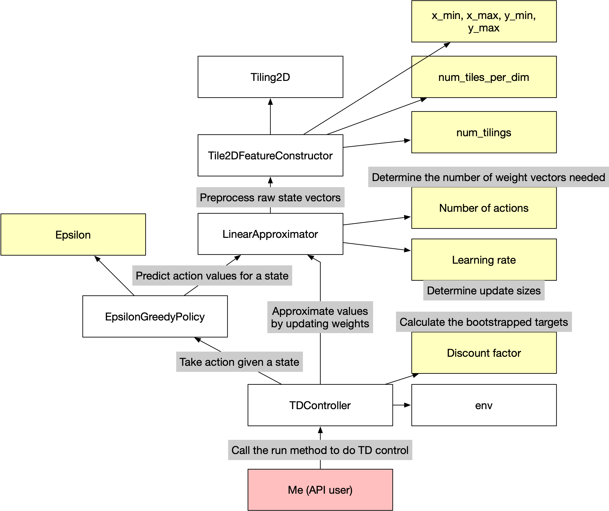
The arrows in the diagram below can be interpreted as "depends on". For example, the LinearApproximator class depends on the Tile2DFeatureConstructor class to preprocess raw state vectors. The white rectangles are classes, the yellow ones are constants, and the red rectangle is me.

# vrepr stands for value representation
vrepr = LinearApproximator(
    num_actions=3,
    lr=0.5/8,
    fc=Tile2DFeatureConstructor(
        x_min=-1.2, x_max=0.5, y_min=-0.07, y_max=0.07,
        num_tiles_per_dim=8, num_tilings=8,
        seed=42
    ),
)
policy = EpsilonGreedyPolicy(vrepr, epsilon=0, actions=[0, 1, 2])
env = gym.make('MountainCar-v0')
td_controller = TDController(env=env, policy=policy, vrepr=vrepr, discount_factor=1)
Since training takes some time, I have saved the training history and resulting weights in the next section. You can uncomment the code cell below to re-train the agent.
# episode_lengths = td_controller.run(500)
Plot episode lengths over time
Save the episode lengths during training.
# with open('episode_lengths.json', 'w+') as json_f:
#     json.dump(episode_lengths, json_f)
Load the episode lengths during training.
with open('episode_lengths.json', 'r') as json_f:
    episode_lengths = np.array(json.load(json_f))
Save the weights after training.
# with open('ws.json', 'w+') as json_f:
#     json.dump([w.tolist() for w in vrepr.ws], json_f)
Load the weights after training.
with open('ws.json', 'r') as json_f:
    ws = [np.array(sublist) for sublist in json.load(json_f)]
vrepr.ws = ws
plt.plot(savgol_filter(episode_lengths, 3, 2))
plt.xlabel('Number of episodes'); plt.ylabel('Episode length')
plt.show()
Watch the car climbs the hill (videos)
ffmpeg may be required to play the videos on Mac OS.
To install it, see
Initial position: left of the lowest point
env = gym.make('MountainCar-v0')

env.seed(42)  # start from the left of the lowest point; seed found by trial-and-error

env = wrappers.Monitor(env, "./video_from_left", force=True)
state = env.reset()

actual_xs_from_left = []
actual_vs_from_left = []

print('Initial state:', state)

for _ in range(1000):
    actual_xs_from_left.append(state[0]); actual_vs_from_left.append(state[1])
    action = policy.act(tuple(state))
    state, reward, done, info = env.step(action)
    if done: break
env.close()
video = io.open('./video_from_left/openaigym.video.%s.video000000.mp4' % env.file_infix, 'r+b').read()
encoded = base64.b64encode(video)
HTML(data='''
    <video width="360" height="auto" alt="test" controls><source src="data:video/mp4;base64,{0}" type="video/mp4" /></video>'''
.format(encoded.decode('ascii')))
Initial position: right of the lowest point
# from gym import wrappers

env = gym.make('MountainCar-v0')

env.seed(50)  # start from the right of the lowest point; seed found by trial-and-error

env = wrappers.Monitor(env, "./video_from_right", force=True)
state = env.reset()

actual_xs_from_right = []
actual_vs_from_right = []

print('Initial state:', state)

for _ in range(1000):
    actual_xs_from_right.append(state[0]); actual_vs_from_right.append(state[1])
    action = policy.act(tuple(state))
    state, reward, done, info = env.step(action)
    if done: break
env.close()
video = io.open('./video_from_right/openaigym.video.%s.video000000.mp4' % env.file_infix, 'r+b').read()
encoded = base64.b64encode(video)
HTML(data='''
    <video width="360" height="auto" alt="test" controls><source src="data:video/mp4;base64,{0}" type="video/mp4" /></video>'''
.format(encoded.decode('ascii')))
Interpret the learned value function
q = np.zeros((100, 100, 3))
xs = np.linspace(-1.2, 0.5, 100)
vs = np.linspace(-0.07, 0.07, 100)
for i, x in enumerate(xs):
    for j, v in enumerate(vs):
        for k, a in enumerate([0, 1, 2]):
            q[i, j, k] = vrepr.calc_q((x, v), a)
xxs, vvs = np.meshgrid(xs, vs)
fig = plt.figure(figsize=(12, 5))

ax = fig.add_subplot(121, projection='3d')
ax.plot_surface(xxs, vvs, -q.max(axis=-1).T, cmap='coolwarm', edgecolors='black', lw=0.6)
ax.view_init(70, -60)

plt.xlabel('Position')
plt.ylabel('Velocity')
ax.set_zlabel('Cost-to-go')
ax.set_title('Cost-to-go (3D visual)')

ax = fig.add_subplot(122)

plt.pcolormesh(xs, vs, -q.max(axis=-1).T, shading='auto', cmap='coolwarm')
ax.scatter([-0.5, -0.5, -0.5], [-0.04, 0, 0.04], s=20, color='black', label='3 states for discussion')
plt.colorbar()

plt.xlabel('Position'); plt.ylabel('Velocity')
plt.title('Cost-to-go (2D visual)')

plt.legend()

plt.tight_layout()
plt.show()
Note that the cost-to-go of a state is simply the negated value of that state.
Here, we attempt to understand the cost-to-go (CTG) function (why it is the way it is) under the learned policy by considering 3 locations in the state space (see "3 states for discussion" in the legend of the RHS plot above).
| State vector | CTG | Potential energy (of car) | Kinetic energy (of car) | Velocity towards the goal? |
|---|---|---|---|---|
| Middle point | Highest | Low (position at -0.5) | Low (zero velocity) | NA |
| Bottom point | Second highest | Low (position at -0.5) | High (non-zero velocity) | No($\star$) |
| Top point | Lowest | Low (position at -0.5) | High (non-zero velocity) | Yes |
($\star$) The car needs to first convert its kinetic energy to potential energy by climbing the left hill and then convert its potential energy back into kinetic energy with velocity in the right direction, which takes some time.
Interpret the learned policy
plt.figure(figsize=(7, 7))

plt.pcolormesh(xs, vs, q.argmax(axis=-1).T, shading='auto', cmap='coolwarm')
plt.plot([-0.5, -0.5], [-0.07, 0.07], '--', color='white')
plt.plot(actual_xs_from_left, actual_vs_from_left, color='orange', linewidth=5, label='Actual trajectory 1')
plt.plot(actual_xs_from_right, actual_vs_from_right, color='lightgreen', linewidth=5, label='Actual trajectory 2')
plt.xlabel('Position'); plt.ylabel('Velocity')
plt.legend()

plt.show()
Here, we attempt the understand the learned policy by looking at two actual trajectories in the state space, one starting from the left of the lowest position (the orange curve) and another starting from the right of the lowest position (the green curve).
The optimal policy is plotted in the background. Blue represents full throttle to the left; grey represents no throttle; red represents full throttle to the right. The white dashed vertical line emphasizes the lowest position.
Let's look at the orange trajectory that starts from the left of the lowest point. From the video in the "Watch the car climbs the hill - Initial position: left of the lowest point" section, we can clearly see that this trajectory is divided up into three phases:
- Phase 1: the car climbs the right hill
- Phase 2: the car goes down the right hill and climbs the left hill
- Phase 3: the car goes down the left hill, climbs the right hill and reaches the terminal condition
These 3 phases are also clearly visible on the plot above.
- In the first phase, the optimal action is almost always full throttle to the right (red).
- In the second phase, the optimal action is almost always full throttle to the left (blue), except for a noticeable period of no throttle at the end of this phase.
- In the third and final phase, the optimal action is almost always full throttle to the right, which, together with the potential energy accumulated by the car, helps the car move all the way to the goal on top of the right hill.
A similar interpretation can be given to the green trajectory.