Back to the list of RL posts.
Dyna-Q
Started by Zhihan on 2020-08-11 20:30:00 +0000.
Time took to write: 8 days.
- What is planning?
- The tabular one-step Dyna-Q algorithm
- The effect of planning on policy learning
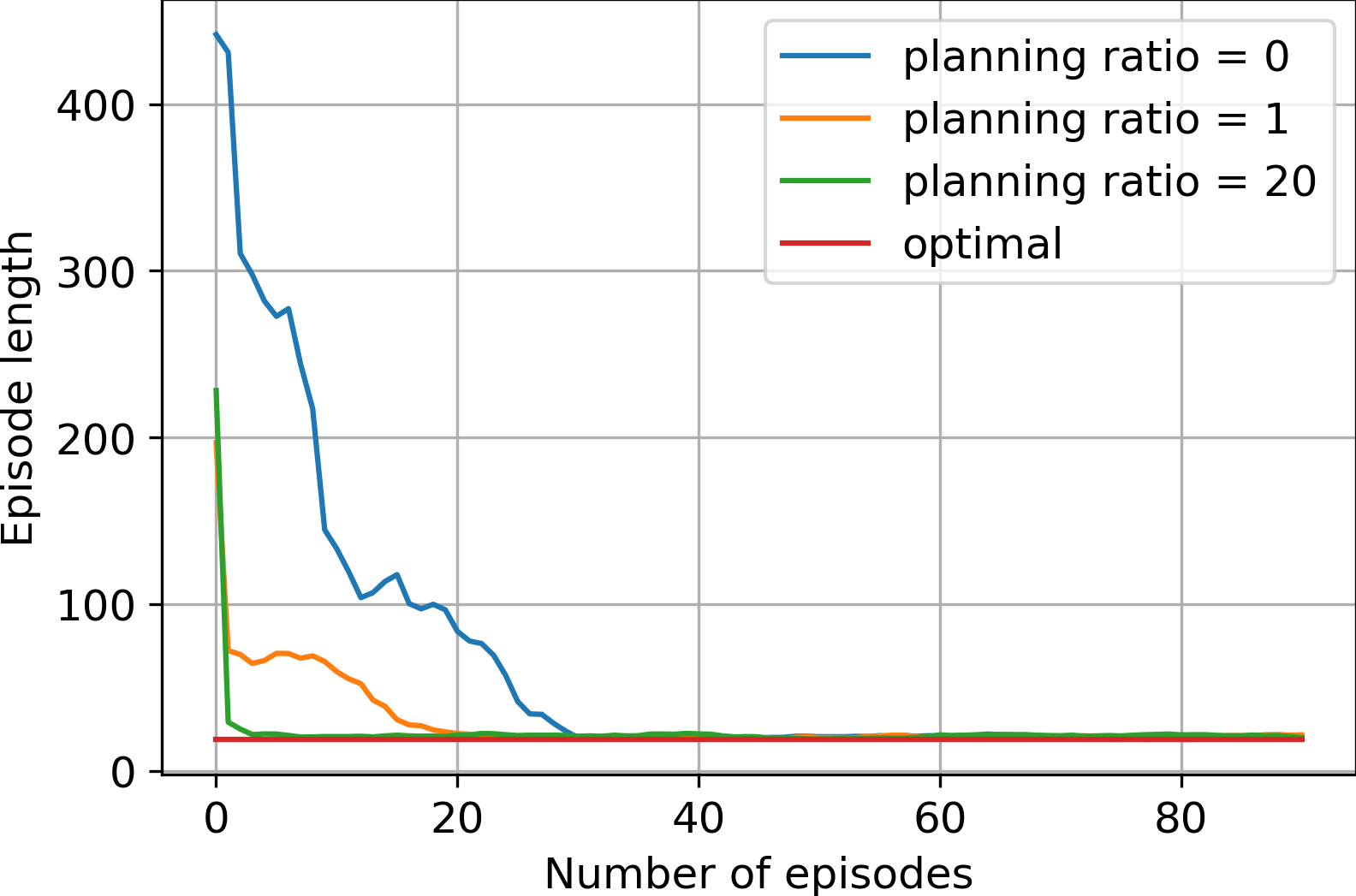
- The effect of different planning ratios on policy learning
- Problems with Dyna-Q
In this post, we learn the basic definition of planning in the context of reinforcement learning, and implement a simple algorithm called Dyna that adds planning to the one-step Q-learning algorithm.
What is planning?
In RL, planning (formally known as state-space plannning) is the evaluation the value function under a policy using simulated experiences generated by the model of an environment (explained shortly). This sounds a lot like learning, the evaluation of the value function under a policy using real experiences. Therefore, they serve the same purpose: in both cases, making the policy greedy or epsilon-greedy with respect to a more accurate value function improves that policy.
A model of the environment is anything that an agent can use to predict how the environment will respond to its actions (i.e., simulate or generate experiences). There are two types of models:
- Distribution models: given a state-action pair, produce all possible next states and their probabilities
- Sample models: given a state-action pair, produce one possible next state
Distribution models are stronger than sample models because they can do everything a sample model can; however, they are generally harder to obtain for many problems.
Sidenote Distribution models might be confusing because a distribution over next states is very different from our concept of experience. A way to understand such models is to view experiences in terms of why we need them in RL: value backup. The value of a state is the expected return following it, and viewing experiences (and thus the corresponding returns) as a distribution help us calculate this expectation. A sample model calculates this same expectation implicitly by sampling individual instances of experience, which make itself more intuitive.
Here’s a flowchart of how planning works:
\[\begin{align*} \text{model (input)} \to \text{simulated experiences} \to \text{values} \to \text{improved policy (output)} \end{align*}\]Here possible relationships between experience, model, values, and policy are summarized below:
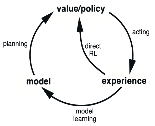
From the diagram above, we that there are at least two roles for real experience:
- Improve the value function and thus policy using the learning methods discussed in previous chapters (via direct RL)
- Improve the model (via model learning)
Note that, in both ways (one direct and one indirect), the value functions and policies are improved. Therefore, these two approaches are also called direct RL and indirect RL.
At this point, we don’t attempt to say whether learning or planning is better - they have deep connections. For example, my other post on TD control emphasizes the link between TD control (a model-free method) and value iteration (a model-based method).
The tabular one-step Dyna-Q algorithm
For illustration purposes, the following version of the algorithm assumes that the environment is deterministic in terms of next states and rewards. If the code between planning: start and planning: end is removed (or if n is set to zero), then we would have the Q-learning algorithm.
Initialize Q(s, a) for all (s, a) pairs with Q(terminal, .) = 0.
Initialize Model to be an empty dictionary.
Initialize VisitedStates to be an empty set.
Initialize ActionsInState to be an empty dictionary.

Set max_episodes.
Set alpha - the learning rate.
Set gamma - the discount factor.
Set n - the planning-learning ratio.

for episode in range(max_episodes):

    Initialize s to be the starting state.

    Loop:

        # ===== learning: start =====

        Choose a using s from the epsilon-greedy (behavior) policy derived from Q.
        Take action a, observe r and s'.

        # preparation for planning

        VisitedStates.add(s)
        if s in ActionsInState.keys():
            ActionsInState[s].append(s)
        else:
            ActionsInState[s] = [a]
        Model[(s, a)] = (r, s')

        Bellman sample = r + gamma * max_a Q(s', a)

        Q(s, a) = (1 - alpha) * Q(s, a) + alpha * Bellman sample  # update rule

        s = s'

        # ===== learning: end =====

        # ===== planning: start =====

        for _ in range(n):

            s = randomly chosen state from VisitedStates
            a = random action chosen from ActionsInState[s]
            r, s' = Model[(s, a)]

            Bellman sample = r + gamma * max_a Q(s', a)

            Q(s, a) = (1 - alpha) * Q(s, a) + alpha * Bellman sample  # update rule

        # ===== planning: end =====

    until s is terminal.
The effect of planning on policy learning
Setup The environment is a 10-by-10 gridworld with a starting state (S) at the top-left corner and a terminal state (T) at the bottom-right corner. All transitions yield zero reward except the ones into the terminal state, which yield a reward of 1. Here, we consider a planning ratio of 20 (20 planning steps per learning step). The learning rate is set to 0.1. The discount factor is set to 0.99 to encourage the agent to find the shortest path(s) to the reward.
Definitions Before we start the discussion, let’s define some terms:
- A learning step: an executation of the update rule in learning section of the pseudo-code above
- A planning step: an executation of the update rule in planning section of the pseudo-code above
- A effective learning step: a learning step that
- modify the value of some state-action pair before value-function convergence, or
- does not change the value of any state-action pair after value-function convergence.
- A effective planning step: a learning step that
- modify the value of some state-action pair before value-function convergence, or
- does not change the value of any state-action pair after value-function convergence.
Observations of the first two episodes During the first episode (before the terminal state is reached), the values of all state-action pairs are zero. This is not surprising because we initialized them to be. If we take a peek at the value function immediately before the first episode finishes (before the learning step happened for the last state-action pair), we would see that the values of all state-action pairs are still zero. Up to this point, no effective learning or planning steps occurred because:
- The values of all state-action pairs are zero.
- The values of all next state-action pairs are zero (a result of the first problem).
- All transitions encountered yield zero reward.
Since the TD error is defined as \(r + \gamma \max_a Q(s', a) - Q(s, a)\) and all three terms above are zero, all TD errors were zero.
After the final timestep of the first episode, the value of one state-action pair (the one encountered on the final timestep) is non-zero due to an effective learning step. If we happen to pick that state-action or any state-action pair that would lead us to that state-action pair, effective planning steps would happen. This is, of course, quite unlikely because there are 396 state-action pairs (99 non-terminal states times 4 actions per state) but planning is done for only 20 randomly-sampled state-action pairs. Indeed, this did not happen.
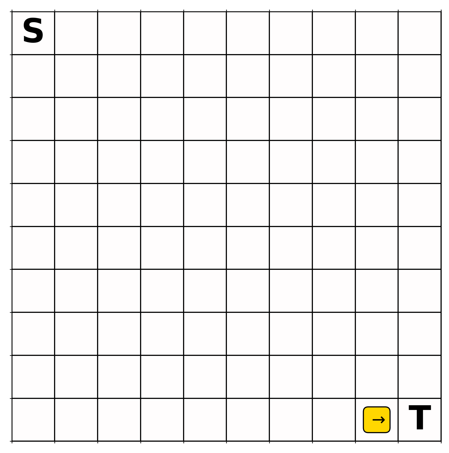
Because zero effective planning steps occurred in the first episode, the greedy action of only one state is defined (Fig. 2), just like in one-step tabular Q-learning; the action values are all zeros for all other states.
Throughout the second episode, there are at most two effective learning steps:
- If the last state-action of the second epsiode is the same as the last state-action of the first episode, then two learning steps occur, one for the last state-action pair, the other for the second last state-action pair.
- If the last state-action of the second epsiode is different from the last state-action of the first episode, then one learning step occurs for the last state-action pair.
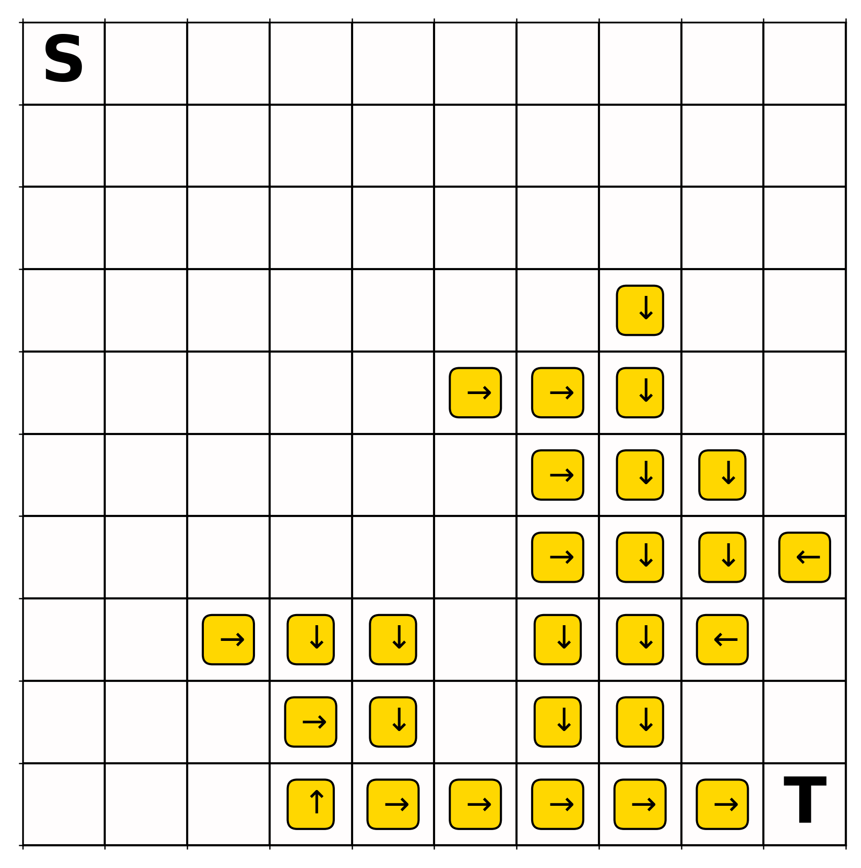
Therefore, if no planning steps occurred, the greedy action would be defined for at most two states. However, if we take a look at Fig. 3, we see that the greedy action is defined for a large proportion of states, and you can following the greedy actions from any of these states all the way to the terminal state. Although many of these greedy actions are not optimal, this is still quite amazing!
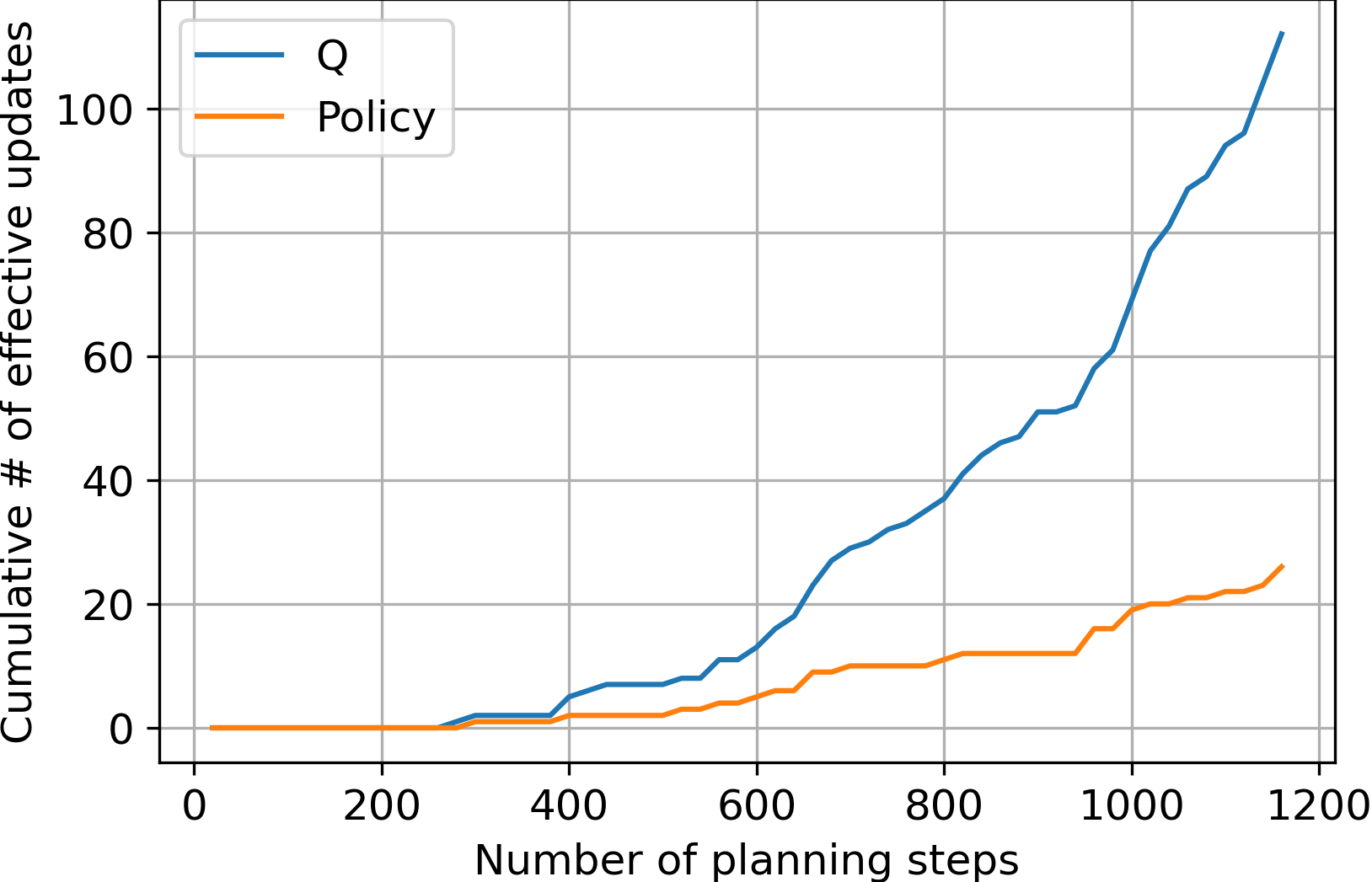
Analysis of the first two episodes To fully understand how planning achieved this, consider the total of number of value updates that happened during the second episode. Under a fixed random seed, the length of the second trajectory is 86, which means 86 learning steps and 1720 planning steps (86 learning steps times a planning ratio of 20). Initially, most planning steps were not effective (see the initial flatness of Fig. 4). Nevertheless, there were a few effective planning steps, the ones for state-action pairs around the terminal state that:
- Have non-zero values
- Lead into state-action pairs with non-zero values
- Lead into the terminal state (\(r=1\))
because, again, the TD error is defined as \(r + \gamma * \max_a Q(s',a) - Q(s, a)\).
As time goes (allowed by a LARGE number of planning steps), the frontier of state-action pairs with non-zero values propagate backwards towards the starting state; as more state-action pairs have non-zero values, the rate of effective planning steps increase (see the increasing slope of Fig. 4). A milder version of the trend applies for the policy as not all changes in the value function is reflected by the policy.
The effect of different planning ratios on policy learning
Problems with Dyna-Q
Efficiency
As shown in Figure 4, the rate of effective value updates is small in the beginning because the values of most state-action pairs are zero and all transitions between most states yield zero reward. In this case, the TD error calculated would be zero for state-action pairs whose value is zero and whose next state-action pairs have zero value. Yet, at the beginning, a uniform selection plan gives a lot of probability to such state-action pairs. Therefore, a lot of useless updates are performed and negligible change in value function or policy is observed at the beginning.
Can we do better than this?
Initially, only state-action pairs (let’s call this group of pairs A) leading into the goal state gets updated after learning from the first episode. Planning should focus on state-action pairs leading into group A or terminal state-action pairs because these pairs have non-zero value or non-zero reward respectively, and then work backward to the starting state(s). In general, however, transitions to goals state don’t necessarily give +1 reward and previous transitions can also yield arbitrary reward. Therefore, we want to work back not just from goal states but from any state whose value has changed significantly.
This idea, which is called backward focusing, is the motivation for the Prioritized Sweeping algorithm, which we shall see in another post. In constrast, forward focusing methods prioritizes updates based on how likely a state-action pair is to appear on actual trajectories and are therefore on-policy. Both methods intend to improve the efficiency of the value-function computation (finding a better solution in shorter time) by distributing or prioritizing updates.
When the model is wrong: Dyna-Q+
So far into the book, we have only considered how to find the optimal policy for a fixed environment. What if the environment changes during the course of training? Would this impact the algorithms’ performance on finding the optimal policy?
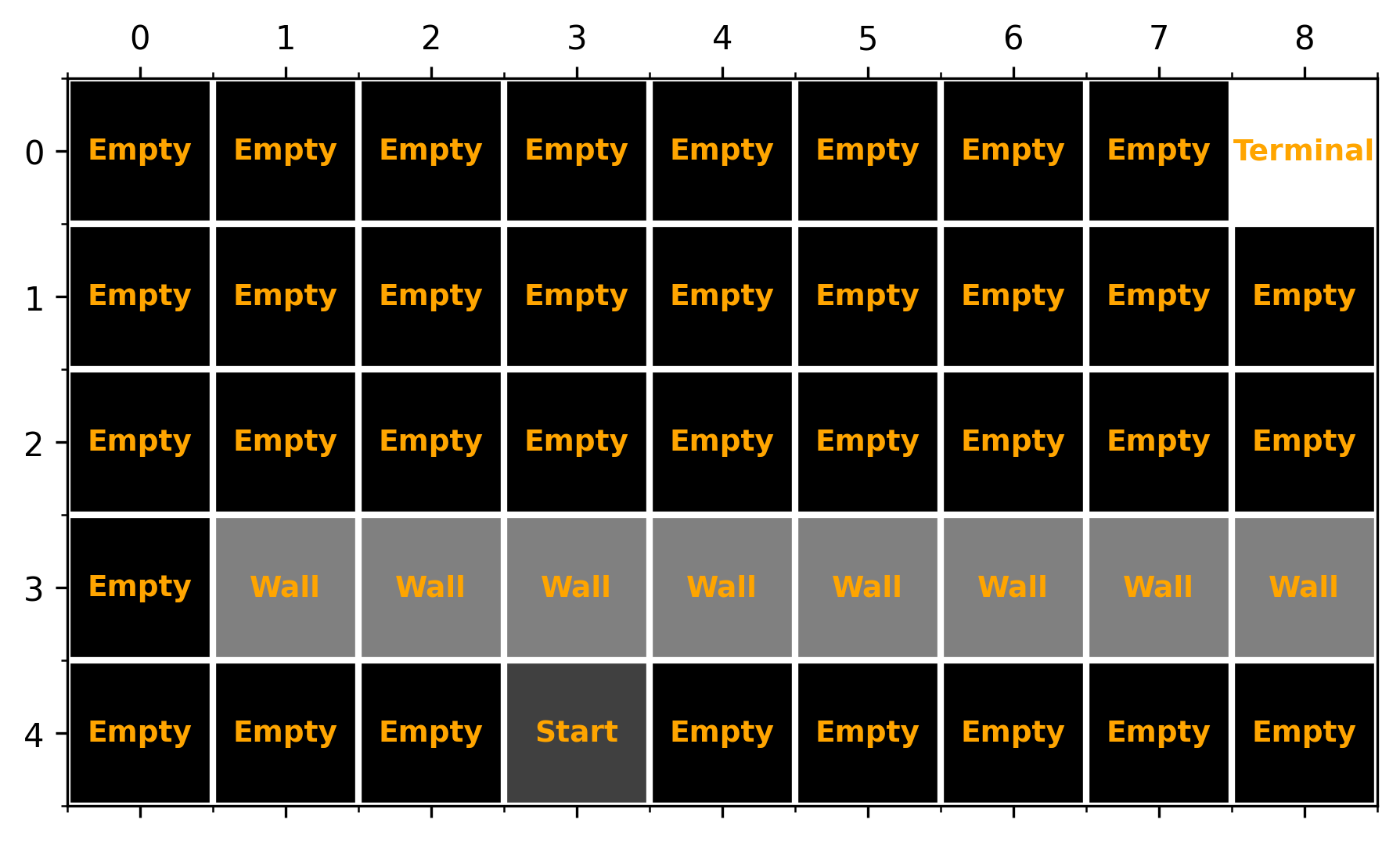
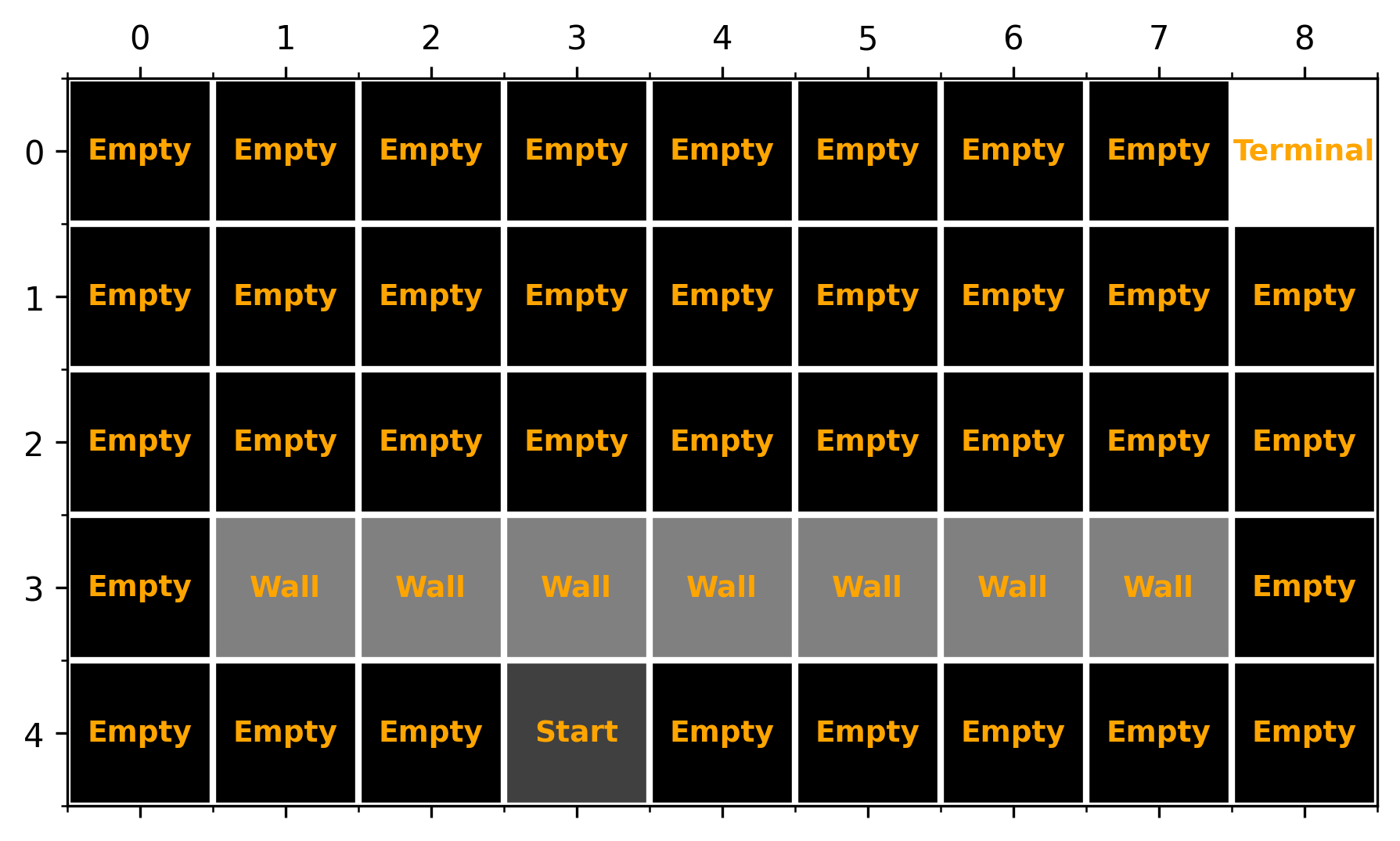
Example To make things concrete, consider the environment in Figure 6. Transitions into the terminal state yield a reward of 1 and all other transitions yield a reward of zero. A discount factor of 0.95 is used for shortest-path finding. Initially, to get from the starting state to the terminal state, the agent needed to go around the walls from the left. After running Dyna-Q for 100 episodes, we suddenly opened up a shorter path (Figure 7) than the shortest path previously available.
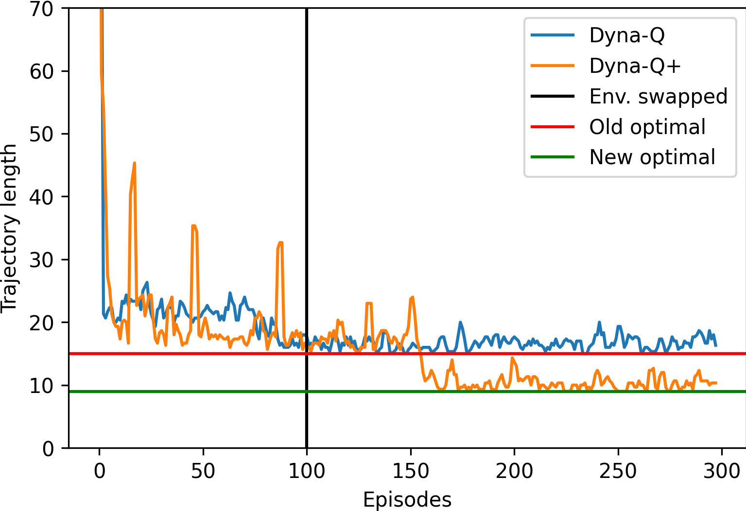
Dyna-Q never discovered this shorter path, while Dyna-Q+ (a modification of Dyna-Q) noticed and continued to exploit it starting from about 50 episodes after the swap (Figure 8). The corresponding policies learned are shown in Figure 9 and 10.
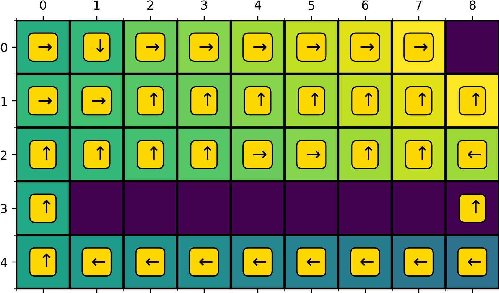
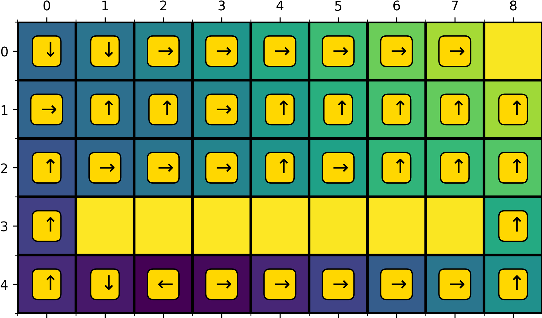
Why does Dyna-Q fail? We will discuss what Dyna-Q+ is in a moment. At this point, simply note that Dyna-Q+ encourages exploration more than Dyna-Q. While all the exploration of Dyna-Q comes from the epsilon-greedy policy, Dyna-Q+ uses an additional heuristic to help the agent explore longer trajectories (consist of multiple sub-optimal actions). As an simple example, under a epsilon-greedy policy with \(\epsilon=0.1\), the probability of taking 3 independent suboptimal actions is almost negligible \((0.1/3)^3 = 0.0000370 \text{ (3 s.f.)}\), assuming that there is one greedy action and three non-greedy actions in each state (common to gridworld). Because of its limited exploration power, the state-action pair ((3, 8), up) is never taken by Dyna-Q and therefore is never added to its model. As a result, ((3, 8), up) appear in neither real nor simulated experiences and it never inherits the high value of the state-action pair ((2, 8), up) right above it. Because ((3, 8), up) is at the frontier of high values (e.g., the value of ((2, 8), up)) and we are using a one-step update rule, when its value is not updated, the values of state-action pairs below it are also not updated.
Problems with Dyna-Q+ However, any exploration comes at the cost of exploitation. As shown in Figure 8, despite having a better max performance, the episode length of Dyna-Q+ can occasionally be very long (represented by the tall spikes) whenever it explores. As a sidenote, it seems to explore periodically.
Does the model cause Dyna-Q’s problem? I don’t think so. If we use SARSA or Q-learning, we will likely have the exact same problem as Dyna-Q. The problem is caused by the fact that epsilon-greedy policy is not good for exploration after some policy has already been learned. If the agent goes into a region currently deemed to have low values, then all actions will ask the agent to move backwards, and a small epsilon can’t help much.
Can model be used to ameliorate the problem (Dyna-Q+)? Yes. The model represents our belief of how the environment works. A simple heuristic to solve the problem is to, in each planning step, use \(r+k \sqrt{\tau}\) instead of \(r\), where \(\tau\) is the number of timesteps (not episodes!) after the state-action pair was last taken and \(k\) is a hyperparameter. This encodes our belief that the environment changes over time and we optimistically expect unseen state-actions to increase their value over time, although this might not be true for every environment out there. The algorithm is shown below.
All modifications (with respect to Dyna-Q) are marked by **********.
Initialize Q(s, a) for all (s, a) pairs with Q(terminal, .) = 0.
Initialize Tau(s, a) for all (s, a) pairs to be zero.  # **********
Initialize Model(s, a) for all (s, a) pairs to be (0, s).  # **********
Initialize States to be a set of all states  # **********
Initialize ActionsInState to be a dictionary mapping actions to states  # **********

Set max_episodes.
Set alpha - the learning rate.
Set gamma - the discount factor.
Set n - the planning-learning ratio.
Set k - the exploration constant.

for episode in range(max_episodes):

    Initialize s to be the starting state.

    Loop:

        for (s, a) in S cross A:  # **********
            Tau(s, a) += 1

        Choose a using s from the epsilon-greedy (behavior) policy derived from Q.
        Take action a, observe r and s'.

        # ===== learn model =====

        Tau(s, a) = 0  # **********
        Model[(s, a)] = (r, s')  # **********

        # ===== do learning =====

        Bellman sample = r + gamma * max_a Q(s', a)
        Q(s, a) = (1 - alpha) * Q(s, a) + alpha * Bellman sample

        s = s'

        # ===== do planning =====

        for _ in range(n):

            s = randomly chosen state from States
            a = random action chosen from ActionsInState[s]

            r, s' = Model[(s, a)]

            exploration bonus = k * sqrt(Tau(s, a))  # **********

            Bellman sample = (r + bonus) + gamma * max_a Q(s', a)  # **********
            Q(s, a) = (1 - alpha) * Q(s, a) + alpha * Bellman sample

    until s is terminal.
Back to the list of RL posts.