Back to the list of RL posts.
On-policy Prediction with Approximation
Started by Zhihan on 2020-08-31 21:30:00 +0000.
- Why approximate value functions?
- How to approximate: supervised learning using SGD
- Linear approximator + feature construction = generalized linear model
- Metric of error for evaluation
- Example
Section headings with stars (*) compare multiple algorithms.
Presentation notes:
- The only concept that is new here is “approximation”; “on-policy” and “prediction” has been discussed by previous sections of the book extensively.
- Follow the table of content instead of reading off my notes directly.
- Starting following my notes more closely starting from the third section.
Why approximate value functions?
In general, the value function is smooth, which means a small change in state leads to a small change in value. Without taking advantage of this observation, the following two issues arise:
- Treating nearby states as if their values are not related at all and updating their values independently slows down learning.
- Some states are not visited at all during training but might show up after deployment. If we don’t interpolate their values using those of the seen states (like what we did in tabular methods), their values would remain randomly initialized. This problem can be particularly serious for high-dimensional state spaces in real-world applications (e.g., lidar data from autonomous vehicles) because states in deployment almost surely never appear in training data.
How we take advantage of the smoothness observation? One way to do so is to approximate the value function using a parameterized functional form such that its number of tunable parameters (or weights) is far less than the number of states. By doing so:
- When weights are updated for a single state, the values of other states also change, hopefully in a good way. If so, rapid learning is achieved.
- Unlike lookup tables, a parameterized value function allows for the evaluation of unseen states. This process is known as generalization and is similar to interpolation.
How to approximate: supervised learning using SGD
Prediction is regression. In a prediction problem, we want to learn a mapping from each state to its expected return (under some policy), the average of all seen returns so far. It happens to be that by minizing the sum of square errors of a approximator with enough capacity (like a neural network) the outputs approximate the conditional averages of the target data (conditioned on input variables). Therefore, we can use an approximator (again, assuming enough capacity) to perform prediction by training it on existing state-return data using the sum of square errors.
SGD is a online method for optimizing the weights of a regression approximator. Stochastic gradient descent (SGD) is simply gradient descent applied to batches of one pair of input and target values. As we mentioned in the last paragraph, we will be using this technique to minimize the sum of square errors.
The SGD update rule:
\[\begin{align*} \mathbf{w}_{t+1} &\leftarrow \mathbf{w}_t - \frac{1}{2} \alpha \nabla \left\{ \left[ G_t - \hat{v}(\mathbf{s}_t, \mathbf{w}_t)\right]^2 \right\} \\ &= \mathbf{w}_t + \alpha \left[ G_t - \hat{v}(\mathbf{s}_t, \mathbf{w}_t) \right] \nabla \left\{ \hat{v}(\mathbf{s}_t, \mathbf{w}_t) \right\} \\ \end{align*}\]where:
- \(\mathbf{w}_t\) is the weight vector at timestep \(t\).
- \(\alpha\) is the learning rate.
- \(\nabla \left\{ \cdots \right\}\) is the gradient of the function inside the curly brackets with respect to \(\mathbf{w}_t\).
- \(G_t\) is a sample return collected from timestep \(t\) to the timestep at which the terminal state is reached.
- \(\hat{v}\) is the function approximator which inputs a state vector \(\mathbf{s}_t\) (which contains the raw features of some state) and a weight vector \(\mathbf{w}_t\) and outputs the predicted value of \(\mathbf{s}_t\).
SGD can be conveniently applied to a linear approximator. We can easily apply the SGD update rule to a linear approximator:
\[\mathbf{w}_{t+1} \leftarrow \mathbf{w}_t + \alpha \left[ G_t - \hat{v}(\mathbf{s}_t, \mathbf{w}_t) \right] \mathbf{s}_t \nonumber \\\]Linear approximator + feature construction = generalized linear model
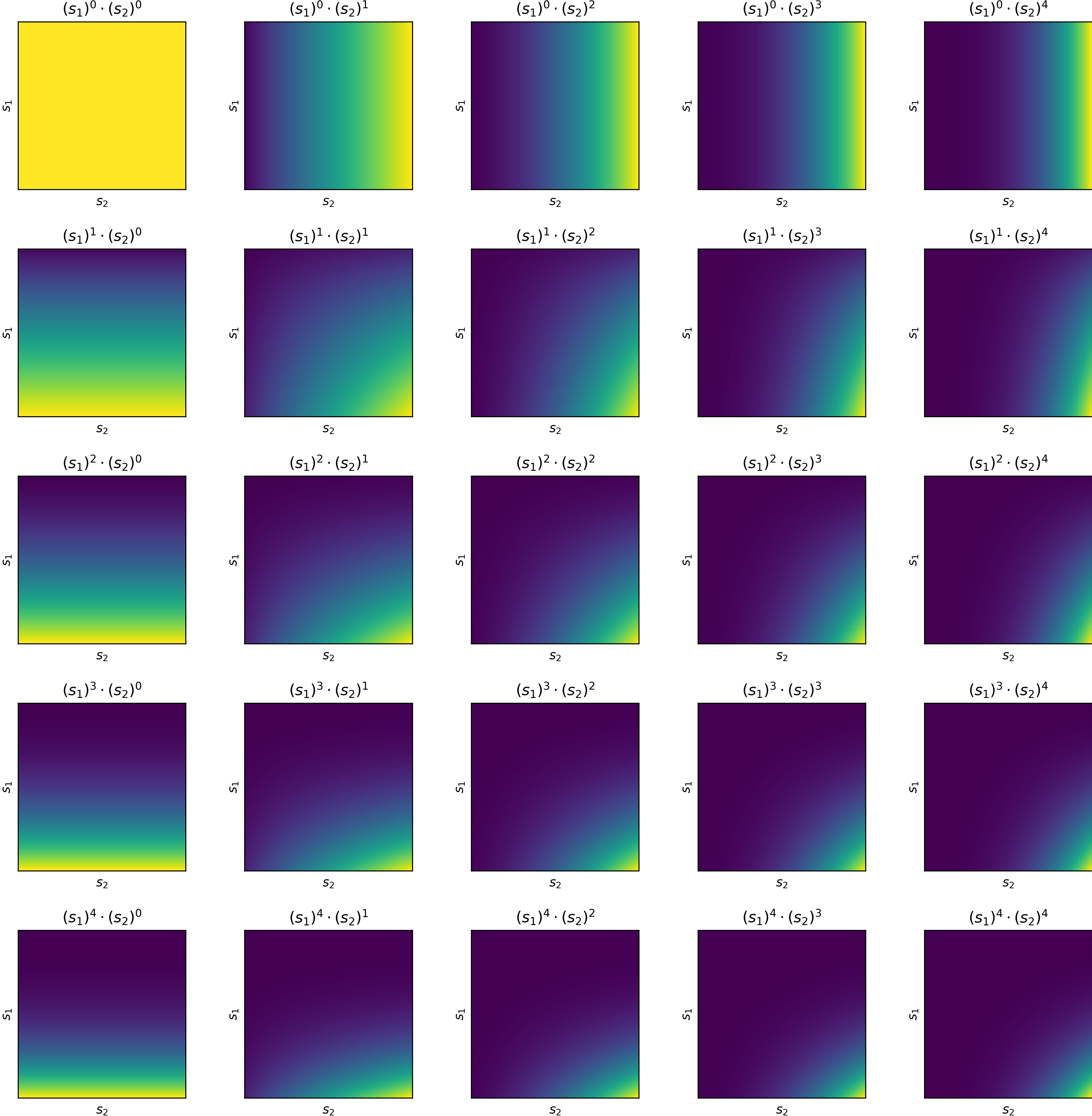
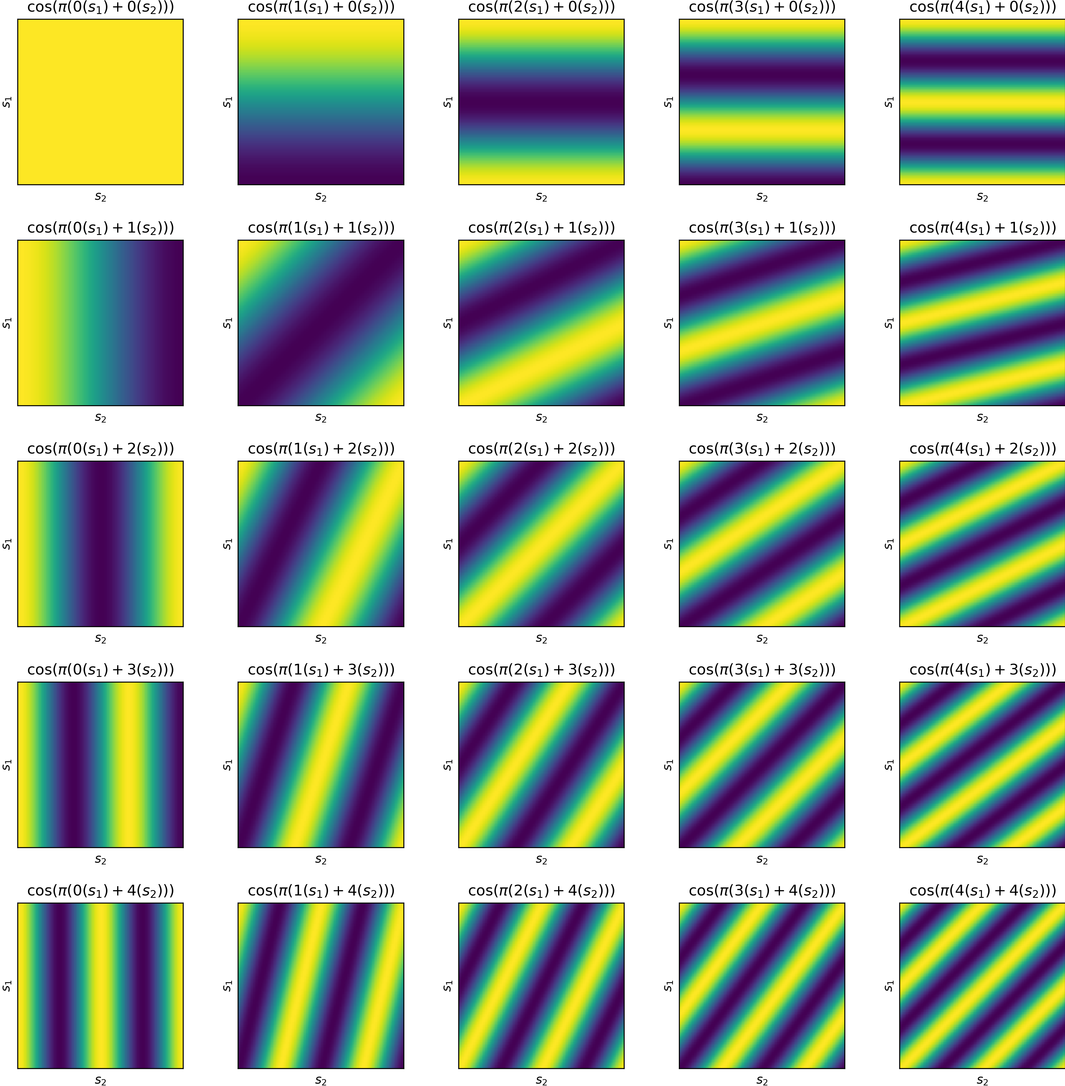
By creating nonlinear transformations of input variables, a linear approximator becomes much more powerful and general. Here are two popular transformations we will consider.
Notes about the figures:
- Origin is placed at the top left corner of each sub-figure.
- Both \(s_1\) and \(s_2\) are normalized to the range \(\left[0, 1\right]\).
Polynomial features

Fourier features

Metric of error for evaluation
It is convenient to measure the degree of error between the approximated values and the true values using, for example, root mean squared error. However, such classical metrics in ML do not reflect the frequency at which states are visited. For example, the value of a state that is never visitied by the policy of interest is in many cases less important than the value of a state that is frequently visited. Therefore, we would like to weigh the error of a state by its probability under the on-policy distribution.
By adding a slight modification to the root mean squares error function, we arrive at the following new error function, the root mean squared value error:
\[\sqrt{\text{VE}} = \sqrt{\sum_{\mathbf{s} \in \mathcal{S}} \mu(\mathbf{s}) \left[v(\mathbf{s}) - \hat{v}(\mathbf{s}, \mathbf{w})\right]^2}\]where \(\mu\) is the on-policy distribution and \(v(\mathbf{s})\) is the true value of the state vector \(\mathbf{s}\).
Note that this metric is merely used for evaluating performance; during training, the sum of squares error is used.
Example
Problem setup
- 20-by-20 gridworld
- Coordinate of the starting state: (0, 0) / top-left corner
- Coordinate of the terminal state: (19, 19) / bottom-right corner
- Reward: all transitions yield a reward of -1 except for those leading into the terminal state, which yields a reward of zero
- Discount factor: 0.90, less than 1 in order to induce curvature in the true value function, making the problem more challenging for function approximators
- Policy to evaluate: the optimal policy (found by policy iteration)
Different MC Algorithms
Basic structure
for _ in range(num_episodes):

  # states and rewards are two lists
  # rewards[t] is the immediate reward of taking the action given by the policy in state[t]

  states, rewards = record_one_trajectory()

  T = len(states) - 1 # last index
  G = 0  # return
  for t in range(T, -1, -1):  # T-1, T-2, ..., 1, 0
    G = self.discount_factor * G + rewards[t]
    value_learner.update(states[t], G)  # different MC algorithms differ in their value_learner
Value learner for tabular MC
class Table:

  def __init__(self, state_space_shape):
    self.sum_of_returns = np.zeros(state_space_shape)
    self.counts = np.zeros(state_space_shape) + 1e-5  # avoid division by zero

  def update(self, state:tuple, target:float) -> None:
    self.sum_of_returns[state] += target
    self.counts[state] += 1

  @property
  def v(self) -> np.array:
    """Return the learned values."""
    return self.sum_of_returns / self.counts
Value learner for gradient MC
class LinearApproximator:

  def __init__(self, lr:float, fc, state_space_shape:tuple):
    self.lr = lr  # learning rate
    self.fc = fc  # feature constructor
    self.w = np.zeros((self.fc.num_features, 1))
    self.state_space_shape = state_space_shape

  def calc_v(self, state:tuple) -> float:
    return float(self.w.T @ self.fc.preprocess(state))

  def calc_grad_wrt_w(self, state:tuple) -> np.array:
    return self.fc.preprocess(state)

  def update(self, state:tuple, target:float) -> None:
    self.w += self.lr * (target - self.calc_v(state)) * self.calc_grad_wrt_w(state)

  @property
  def v(self) -> np.array:
    v = np.zeros(self.state_space_shape)
    for row_ix in range(self.state_space_shape[0]):
      for col_ix in range(self.state_space_shape[1]):
        state = (row_ix, col_ix)
        v[state] = self.calc_v(state)
    return v
Root value error over time*
The root mean squared value error requires the on-policy distribution. While this can be collected during training, I find the errors more meaningful and interpretable when the on-policy distribution is approximated before training happens.
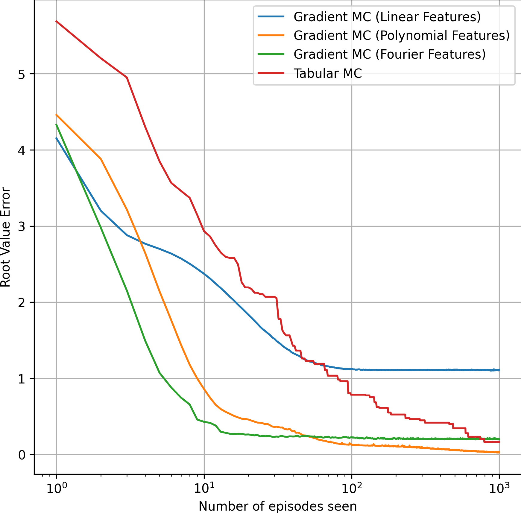
Some important observations of the plot below:
- Initially, although all gradient MC methods had a learning rate of only 0.01, their errors dropped faster than the tabular MC method.
- Between 10 and 100 episodes, the error of the tabular method dropped below the gradient MC method using linear features (due to the limited representation power of linear features).
- Finally, right before reaching 1000 episodes, the error of the tabular method dropped below the gradient MC method using Fourier features, despite the fact that Fourier features led to the fastest initial learning.
- After 1000 epsiodes, the gradient MC method using polynomial features still won the tabular method.

Learned values*

Back to the list of RL posts.