Back to the list of RL posts.
Policy Iteration in Practice
Started by Zhihan on 2020-07-21 16:30:00 +0000.
- Introduction
- Book: Yes, but use either discounting or non-deterministic policy.
- Me: I would like to learn a deterministic policy without using discounting.
- Gallery
Introduction
Algorithms introduced in Chapter 5 (Monte-Carlo methods) and Chapter 6 (TD methods) of Sutton & Barto 2018 approximate the optimal q-table to achieve control. Since these methods were a bit hard to debug and only converge in the limit, I needed a tool to compute the exact optimal q-table to evaluate their performance. Therefore, I went back to Chapter 4 (dynamic programming) and implemented the policy iteration algorithm using q-tables with this question in mind:
Can policy iteration be used to learn optimal deterministic policies and their corresponding optimal value functions?
I also show some galleries of learned value functions in the end along with their source code.
Book: Yes, but use either discounting or non-deterministic policy.
In many problems, our goal is to learn the optimal deterministic policy. This is because deterministic policies perform optimally all the time and thus obtain the highest reward.
Policy iteration is an algorithm that allows us to find the optimal policy and the optimal value function in the limit. It consists of two sub-algorithms: policy evaluation and policy improvement. Certain requirements need to be met for policy evaluation to work. Here’s a relevant quote from section 4.1 of Sutton & Barto 2018:
The existence and uniqueness of \(v_{\pi}\) are guaranteed as long as either \(\gamma < 1\) or eventual termination is guaranteed from all states under the policy \(\pi\).
To understand this quote, let’s consider an example.
Environment
For simplicity, suppose there are only two states in a gridworld: one start state and one terminal state. The start state is on the left of the terminal state. Legal actions in non-terminal states (in this case, the start state only) are up, right, down and left and each action costs a reward of -1. After the agent arrives at the terminal state, the episode terminates and no further rewards are incurred. If the agent takes an action that makes itself outside of the gridworld, it is moved back to its last grid cell and receives a reward of -1.
Initial q-table
To solve this problem, we store the value of each state-action pair (i.e., store the q-table) and do policy iteration.
Suppose we use \(\gamma = 1\) and the agent’s policy is deterministic. First, we randomly initialize the q-table, which is the initial uninformed estimate of the true q-table given the environment and the policy. Then we set the agent’s policy to be greedy with respect to this q-table.
Suppose this q-table looks like this:
| State | Action | Q-value |
|---|---|---|
| start state | up | 0.15 |
| start state | right | -0.09 |
| start state | down | 0.015 |
| start state | left | -0.2 |
Policy-evaluation update formula
First, we do policy evaluation. Note that the agent’s policy is NOT updated at all during this procedure. Let’s derive an update rule for policy evaluation. The relationship between \(V_{\pi}\) and \(Q_\pi\) is listed below:
\[V_{\pi}(s) = \sum_{a} \pi(a \mid s) Q_{\pi}(s, a)\] \[Q_{\pi}(s, a) = \sum_{s', r} p(s', r \mid s, a) \left[ r + \gamma V_{\pi}(s) \right]\]Since we store the q-table, we would like both the LHS and RHS to be expressed in terms of \(Q_\pi\). To do this, we substitue equation 1 into equation 2 and get:
\[Q_{\pi}(s, a) = \sum_{s', r} p(s', r \mid s, a) \left[ r + \gamma \sum_{a'} \pi(a' \mid s') Q_{\pi}(s', a') \right]\]which can be easily turned into the following update rule:
\[Q_{\pi}(s, a) \leftarrow \sum_{s', r} p(s', r \mid s, a) \left[ r + \gamma \sum_{a'} \pi(a' \mid s') Q_{\pi}(s', a') \right]\]We say policy evaluation has convergenced when the LHS and the RHS of the update rule above is the same. In other words, the stepsize of each update needs to converge to zero.
No discounting and deterministic policy
Since (state, up) has the highest initial value, the policy always instruct the agent to move up when the agent is in the start state. However, moving up in start state, according to the rules of this environment, return the agent back to the start state and the story repeats for an infinite number of times. Therefore, the true value of (state, up) given the environment and the current policy is negative infinity.
The corresponding update rule looks like this:
\[Q_{\pi}(\text{start}, \uparrow) \leftarrow (-1) + Q_{\pi}(\text{start}, \uparrow)\]which clearly drives \(Q_\pi(\text{start}, \uparrow)\) to negative infinity if repeated for an infinite number of times. However, in this case, we cannot check for convergence because the stepsize is always one.
Discounting and deterministic policy
Warning: This analysis here is not meant to be exhaustive. I haven’t looked at the formal proof of why policy evaluation requires either discounting or non-deterministic policy. Nevertheless, I hope they give you a good intuition on why things work / not work.
The true value of \(Q_\pi(\text{start}, \uparrow)\): \((-1) + \gamma(-1) + \gamma^2 (-1) + \cdots = \sum_{k=0}^{\infty} \gamma^k (-1) = \frac{(-1)}{1 - \gamma}\)
The corresponding update rule looks like this:
\[Q_{\pi}(\text{start}, \uparrow) \leftarrow (-1) + \gamma Q_{\pi}(\text{start}, \uparrow)\]The first estimate is related to the initial estimate by the expression:
\[Q_{\pi}^1(\text{start}, \uparrow) = (-1) + \gamma Q_{\pi}^0(\text{start}, \uparrow)\]The second estimate is related to the initial estimate by the expression:
\[\begin{align} Q_{\pi}^2(\text{start}, \uparrow) &= (-1) + \gamma Q_{\pi}^1(\text{start}, \uparrow) \\ &= (-1) + \gamma \left[ (-1) + \gamma Q_{\pi}^0(\text{start}, \uparrow) \right] \\ &= (-1) + \gamma (-1) + \gamma^2 Q_{\pi}^0(\text{start}, \uparrow) \end{align}\]In general, the \(n\)-th estimate is related to the initial estimate by the expression:
\[Q_{\pi}^n(\text{start}, \uparrow) = \sum_{k=0}^{n-1} \gamma^{k} (-1) + \gamma^n Q_{\pi}^0(\text{start}, \uparrow)\]As \(n\) reaches infinity:
\[Q_{\pi}^{\infty}(\text{start}, \uparrow) =\sum_{k=0}^{\infty} \gamma^{k}(-1) = \frac{-1}{1 - \gamma}\]We just showed that the estimated value converge to the true value in the limit.
Now consider the upper bound on the difference between the true value and the \(n\)-th estimated value:
\[\begin{align} \left\vert Q_{\pi}^{\infty}(\text{start}, \uparrow) - Q_{\pi}^n(\text{start}, \uparrow) \right\vert &= \left\vert \sum_{k=0}^{\infty} \gamma^{k}(-1) - \sum_{k=0}^{n-1} \gamma^{k} (-1) - \gamma^n Q_{\pi}^0(\text{start}, \uparrow) \right\vert \\ &= \left\vert \sum_{k=n}^{\infty} \gamma^{k}(-1) - \gamma^n Q_{\pi}^0(\text{start}, \uparrow) \right\vert \\ &\leq \left\vert \sum_{k=n}^{\infty} \gamma^{k}(-1) \right\vert + \left\vert \gamma^n Q_{\pi}^0(\text{start}, \uparrow) \right\vert \end{align}\]As \(n\) increases, this upper bound decreases at a decreasing rate (a bit mouthful but it’s true). This shows that, unlike in the last setting we considered, the stepsize decreases as we approach the goal. This allows us to stop policy iteration when the difference between the RHS and the LHS of the update rule reaches some preset precision tolerance.
Hint for deriving the upper bound: \(\left\vert a - b \right\vert = \left\vert a + (-b) \right\vert \leq \left\vert a \right\vert + \left\vert -b \right\vert = \left\vert a \right\vert + \left\vert b \right\vert\)
No discounting and epsilon-greedy policy
The corresponding update rule looks like this:
\[Q_{\pi}(\text{start}, \uparrow) \leftarrow (-1) + (1 - \epsilon)Q_{\pi}(\text{start}, \uparrow) + \frac{\epsilon}{\mid A \mid} \left[ Q_{\pi}(\text{start}, \uparrow) +Q_{\pi}(\text{start}, \rightarrow) + Q_{\pi}(\text{start}, \downarrow) + Q_{\pi}(\text{start}, \rightarrow) \right]\]where \(\epsilon\) is the probability assigned to picking a random action (the greedy action can still be picked by chance).
Note that I won’t go into any derivation here because the update rule is a lot more complicated, but the main ideas are still the same.
- First, the true value must be finite.
- Second, the estimated value converges to the true value in the limit.
- Third, the difference between the true value and estimated value decreases at a decreasing rate, so policy evaluation can be terminated early on after the difference between the RHS and the LHS of the update rule is lower than some precision tolerance.
Me: I would like to learn a deterministic policy without using discounting.
Personally, I find neither of these approaches satisfactory.
- Discounting is mathematically convenient, but it seems to a bit artificial. For example, in the gridworld setting, without discounting, the value of state-action pair tells us the exact number of actions to take to get to terminal state, given that the reward of every action is -1; however, if we use discounting, this interpretation is not valid anymore.
- Why learn a epsilon-greedy policy when we want a greedy policy more badly?
Here are some of my attempts that use \(\gamma=1\) and learn a deterministic policy. Both of them worked in practice.
Approach 1: Decay epsilon of the epsilon-greedy policy
Start with \(\gamma=1\) and an epsilon-greedy policy. During each policy improvement step, decay epsilon by multiplying it by a constant like 0.8 or 0.9. Check for convergence to optimal value function and optimal policy using the Bellman’s optimality equation for epsilon-greedy policies. Eventually, epsilon becomes so small so that the epsilon-greedy policy is essentially a deterministic policy.
Approach 2: Truncate policy evaluation
This really came as a surprise. When trying approach 1 for large gridworlds (10 by 10), I find that the first round policy evaluation takes forever, so I allowed a larger precision tolerance. The larger this tolerance was, the fast the algorithm ran. Then I thought, the use of very large policy-evaluation tolerance is essentially to truncated policy evaluation, which was mentioned briefly in the value iteration section of the book.
Out of curiosity, I tried truncated policy evaluation starting from a greedy policy directly, and everything worked like a charm! This approach converged at least 5 times faster than approach 1. My implementation alternatives between truncated policy evaluation (one value update for all state-action pairs) + policy improvement.
This might be why it works so well: truncated policy iteration relies on the fact that policy improvement can avoid a state-action pair as long as the value of that pair is lower than other pairs; it does not need to know that the return for that pair is negative infinity.
Gallery
Note the difference between and conv_tol in the following examples. pe_tol is the precision tolerance for policy evaluation, while conv_tol is the precision tolerance for convergence of policy iteration. pe_tol is the maximum difference allowed between the LHS and the RHS of the update rule (which is really just the Bellman equation), while conv_tol is the maximum difference allowed between the LHS and RHS of the Bellman optimality equation. More details are available from the notebook and the documentation.
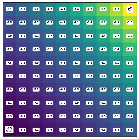
Book’s first approach: discounting
# very fast

policy = EpsilonGreedyPolicy(q=q_initial_estimate, epsilon=0)

algo = PolicyIteration(
    env=env, policy=policy,
    discount_factor=0.9,
    truncate_pe=False, pe_tol=1e-1,
    conv_tol=1e-16
)

Book’s first approach: epsilon-greedy policy
# very, very, very slow
# probably for the same reason mentioned in section "No discounting and deterministic policy"

policy = EpsilonGreedyPolicy(q=q_initial_estimate, epsilon=0.1)

algo = PolicyIteration(
    env=env, policy=policy,
    discount_factor=1,
    truncate_pe=False, pe_tol=1e-1,
    conv_tol=1e-16
)
It was so slow that I didn’t bother waiting for the results. I did verify that the policy evaluation error was decreasing.
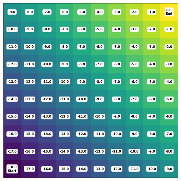
My second approach
# very fast

policy = EpsilonGreedyPolicy(q=q_initial_estimate, epsilon=0)

algo = PolicyIteration(
    env=env, policy=policy,
    discount_factor=1,
    truncate_pe=True, pe_tol=None,
    conv_tol=1e-16
)

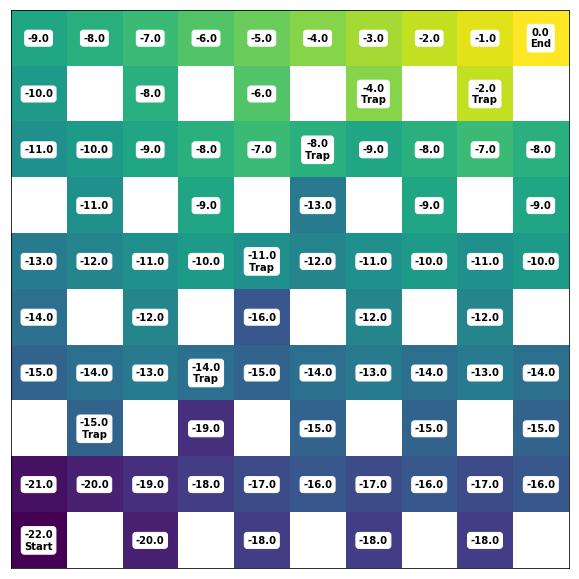
Here’s a more sophicated environment with walls and traps (large negative rewards of -5):

Back to the list of RL posts.