Back to the list of RL posts.

SARSA vs. Q-Learning

Started by Zhihan on 2020-07-25 23:00:00 +0000.

Theory
- Value iteration
- Asychronous dynamic programming
Practice

Theory

This post discusses the intuition of SARSA and Q-learning, which in my opinion is missing from Sutton & Barto (2018).

Value iteration

To motivate the TD control algorithm, it is convenient to begin with the value iteration algorithm (the extreme version of truncated policy iteration):

Initialize \(Q(s, a)\) for all \((s, a)\) pairs arbitrarily except that \(Q(\text{terminal}, \cdot) = 0\).
Loop through all \((s, a)\)’s:
- Do \(q_{\pi}(s, a) \leftarrow \sum_{s’, r} p(s’, r \mid s, a) \left[ r + \sum_{a'} \pi(a' \mid s’) q_{\pi}(s’, a’) \right]\).
- Update \(\pi\) with respect to \(q_{\pi}(s, a)\).
Until \(q_{\pi}(s, a)\) has converged to \(q_{\ast}(s, a)\) or \(\pi\) is stable.

The value iteration algorithm makes the following assumptions:

All the state-action pairs are known (otherwise we won’t be able to loop through them in an organized fashion).
All state-action pairs are updated with the same frequency.
The dynamics of the environment \(p(s’, r \mid s, a)\) is known.

Asychronous dynamic programming

The concept of asynchronous DP is the bridge from value iteration to one-step temporal-difference methods. From Sutton & Barto (2018):

Asynchronous DP algorithms are in-place iterative DP algorithms that are not organized in terms of systematic sweeps of the state set. These algorithms update the values of states in any order whatsoever, using whatever values of other states happen to be available. The values of some states may be updated several times before the values of others are updated once. To converge correctly, however, an asynchronous algorithm must continue to update the values of all the states: it can’t ignore any state after some point in the computation.

This means that, instead of sweeping systematically, we can simply use an epsilon-greedy policy to “encounter” all state-action pairs and update their value as they are encountered. Assumption 1 and 2 are removed.

The update rule can be used to evaluate a target policy (which we shall denote by \(\pi\)) that is different from the behavior policy (which we shall denote by \(b\)). This is because the mere purpose of the behavior policy, just like systematic sweeping in value iteration, is to encounter all state-action pairs.

Nevertheless, a behavior policy that assigns the most probability to actions that are also the most probable under the target policy would visit the state-action pairs that are more relevant to optimal behavior more often.

Assumption 3 can be removed by making both the outer (and inner expectation) of the update rule implicit through sampling:

Previously: \(q_{\pi}(s, a) \leftarrow \sum_{s’, r} p(s’, r \mid s, a) \left[ r + \sum_{a'} \pi(a' \mid s’) q_{\pi}(s’, a’) \right]\)
Now: \(q_{\pi}(s, a) \leftarrow \text{the average of all samples (with more weight given to recent ones)}\)
- Each sample looks like \(r + q_{\pi}(s’, \pi(s'))\), where \(r\) is the actual reward received by taking \(a\) in \(s\) and \(s’\) is the actual next state reached by the policy by taking \(a\) in \(s\). For convenience, let’s just call this the Bellman sample.

If \(b=\pi\), we have SARSA. SARSA is on-policy because it is behaving according to and evaluating the same policy.

If \(\pi\) is a greedy policy, we have Q-learning. Q-learning is off-policy because it evaluates a target policy that is different from the behavior policy used for acting.

If the inner expectation is explicit, we have expected SARSA.

The practical differences between SARSA and Q-learning will be addressed later in this post.

Practice

Incremental implementation

Before outlining the pseudocode of SARSA and Q-learning, we first consider how to update an average \(A_{n+1}\) in an online fashion using an one-step-older average \(A_n\) and a newly available sample \(a_{n}\).

\[\begin{align*} A_{n+1} &= \frac{1}{n} \sum_{i=1}^n a_i \\ &= \frac{1}{n} \left( a_n + \sum_{i=1}^{n-1} a_i \right) \\ &= \frac{1}{n} \left( a_n + (n-1) \frac{1}{n-1} \sum_{i=1}^{n-1} a_i \right) \\ &= \frac{1}{n} \left( a_n + (n-1) A_{n} \right) \\ &= \frac{1}{n} \left( a_n + nA_{n} - A_n \right) \\ &= A_{n} + \frac{1}{n} \left[ a_n - A_n \right] \\ \end{align*}\]

The assumption made by the incremental implementation above is that all samples are obtained from the distribution whose mean is what we want to estimate. Under the framework of general policy iteration, the distribution of returns is always changing since we alternate between evaluating the value function of the current policy and improving the current policy by setting the most probable action to be greedy to that value function. As a result, recent Bellman samples are more relevant than old ones. Therefore, we want to give newer updates more weight. This can be done by changing \(\frac{1}{n}\) to a constant stepsize \(\alpha\) that lies within the interval (0, 1]:

\[\begin{align*} A_{n+1} \leftarrow A_n + \alpha (a_n - A_n) \end{align*}\]

Here’s a perhaps more intuitive way of rewriting this update rule:

\[\begin{align*} A_{n+1} \leftarrow (1 - \alpha) A_n + \alpha a_n \end{align*}\]

Pseudocode of SARSA and Q-learning

Initialize Q(s, a) for all (s, a) pairs with Q(terminal, .) = 0.
Set alpha.
Set mode to either SARSA or Q-learning.

Loop for each episode:
    Initialize s to be the starting state.
    Loop:
        
        Choose a from the epsilon-greedy (behavior) policy derived from Q.
        Take action a, observe s' and r.
            
        If mode is SARSA:
             Choose a' from the epsilon-greedy (target) policy derived from Q.
        If mode is Q-learning:
             Choose a' from the greedy (target) policy derived from Q.
            
        Bellman sample = r + Q(s', a')
        
        Q(s, a) = (1 - alpha) * Q(s, a) + alpha * Bellman sample

        s = s'
    
    until s is terminal.

Cliff-walking experiment

Environment

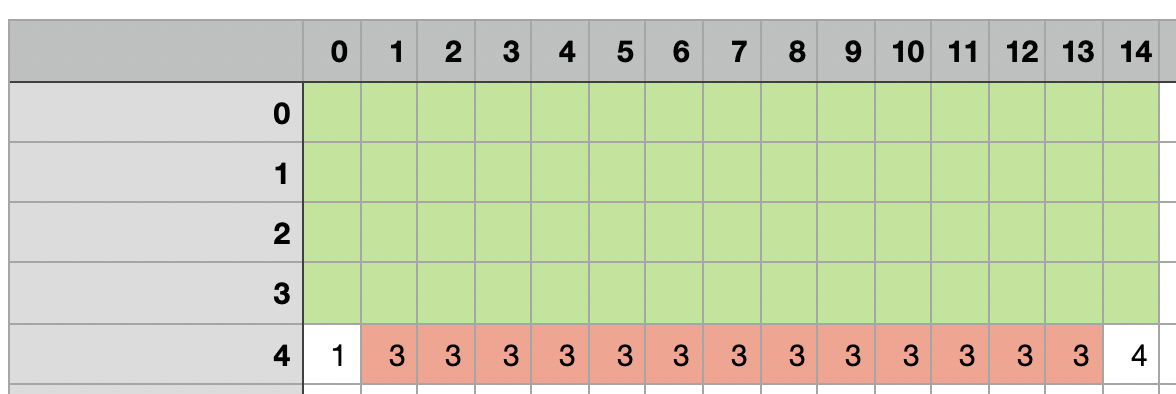
One way to understand the practical differences between SARSA and Q-learning is running them through a cliff-walking gridworld. For example, the following gridworld has 5 rows and 15 columns. Green regions represent walkable squares. Here’s the mapping from index to meaning:

1: the starting state
4: the terminal state (stepping into this causes an epside to terminate; the policy is sent back to the starting state)
3: traps (stepping into a trap causes a -100 reward; the policy continue to take actions from this state though)

Other than traps, stepping into a square incurs a reward of -1.

Online performance

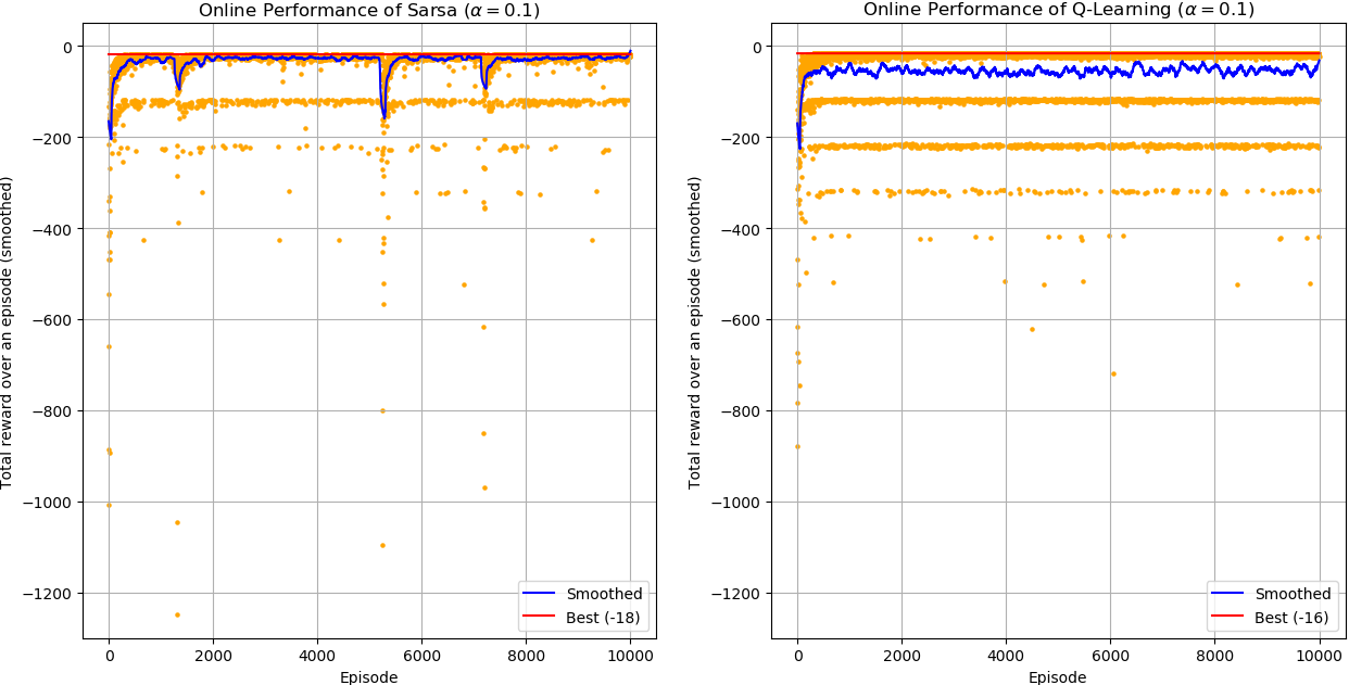
Online performance is the performance of the behavior policy. Here are some important observations:

Q-Learning’s best performance is optimal (the best possible) but SARSA’s best performance is not.
In terms of smoothed performance, SARSA is better than Q-learning most of the times.
SARSA occasionally have sudden drops in performance.

Now, let’s try to understand the intuition behind these observations.

In-depth explanation of online performance

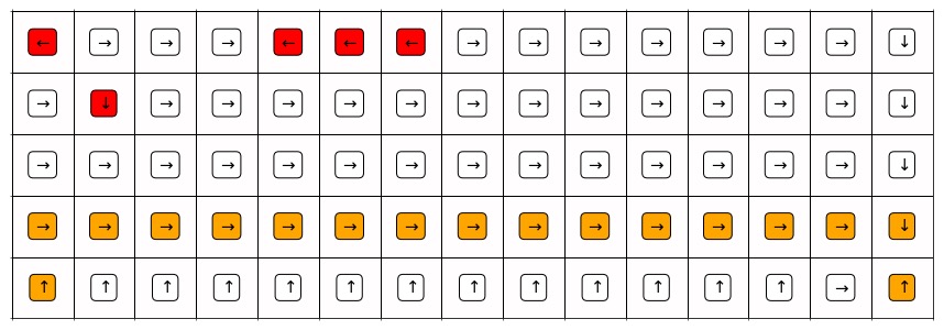
Just like policy iteration / value iteration, Q-learning learns the value of the optimal greedy policy, which travels around the cliff as follows. However, during training (online), the total reward per episode is collected by the behavior policy, which is epsilon-greedy. When the behavior policy tries to walk around the cliff, its randomness can easily cause it to take an suboptimal action into a trap.

Figure 1. The greedy trajectory learned by Q-learning.

Legend:

Orange: grids that are on the learned greedy trajectory
Red: grids at which the learned greedy policy behaves sub-optimally (with respect to a policy-iteration baseline)

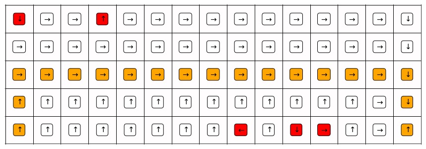
On the other hand, SARSA takes this randomness into account because it learns the value of the behavior policy. Therefore, it uses extra 2 actions, one at the beginning of trajectory and another at the end, to exchange for a safer path.

Figure 2. The greedy trajectory learned by SARSA.

Explanations:

Q-learning’s best performance is optimal but SARSA’s best performance is not.
- For reasons explained above, Q-learning learns the optimal greedy trajectory while SARSA doesn’t. Although Q-learning’s behavior policy is epsilon-greedy, while training, it is still possible for the behavior policy to always take greedy actions over an entire trajectory. When this happens, the total return of the trajectory is optimal.
In terms of smoothed performance, SARSA is better than Q-learning most of the times.
- Both Q-learning and SARSA uses the same epsilon-greedy behavior policy. However, the behavior policy of Q-learning walks closer to the traps and thus it is more likely to take an action into a trap due to randomness and receive a -100 reward.
SARSA occasionally have sudden drops in performance.
- The behavior policy takes greedy actions most of the times and take random actions by 10% of the times.
- This means that the state-action pairs on the greedy trajectory are encountered and evaluated more often; the number of evaluations for surrounding grids fall off exponentially as their distances to the greedy trajectory increase.
- For SARSA, traps are 1 grid away from the greedy trajectory.
- For Q-learning, traps are right next to the greedy trajectory.
- For this reason, Q-learning evaluates actions in traps much frequently (Figure 3) and the greedy actions in all traps are upwards (also optimal) (Figure 1), which will lead the agent immediately out of the trap.
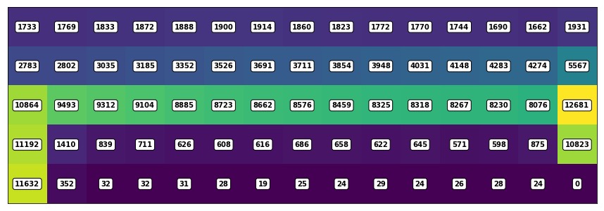
- On the other hand, SARSA evaluates actions in traps only occasionally (Figure 4) and, even after 10000 episodes of training, the greedy actions for three traps are non-optimal* (Figure 1), which will lead the agent into another trap.
- To put everything in a nutshell, although SARSA encounter less traps on average, when it does encounter one, it is more likely encounter several other traps because some actions in traps have incorrect values and thus the corresponding greedy actions are non-optimal*.

*with respect to the environment and the epsilon-greedy behavior policy

Figure 3: Number of evaluations for each state after running 10000 episodes of Q-learning.

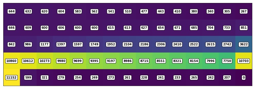
Figure 4: Number of evaluations for each state after running 10000 episodes of SARSA.

Back to the list of RL posts.